Have you looked at the North Pole lately?

• Published: 22 January 2024

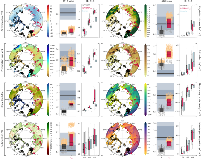
Towards an increasingly biased view on Arctic change​

• Efrén López-Blanco,
• Elmer Topp-Jørgensen,
• Torben R. Christensen,
• Morten Rasch,
• Henrik Skov,
• Marie F. Arndal,
• M. Syndonia Bret-Harte,
• Terry V. Callaghan &
• Niels M. Schmidt

Nature Climate Change volume 14, pages 152–155 (2024)Cite this article

• 9416 Accesses
• 1 Citations
• 658 Altmetric
• Metrics details

Abstract​

The Russian invasion of Ukraine hampers the ability to adequately describe conditions across the Arctic, thus biasing the view on Arctic change. Here we benchmark the pan-Arctic representativeness of the largest high-latitude research station network, INTERACT, with or without Russian stations. Excluding Russian stations lowers representativeness markedly, with some biases being of the same magnitude as the expected shifts caused by climate change by the end of the century.

Main

As a result of the Russian attack on Ukraine, the Western world has excluded Russia from international fora. This geopolitical conflict severely challenges transnational collaboration on global issues. This is particularly evident when it comes to the Arctic. Russia is geographically the largest Arctic nation and is, hence, also one of eight nations within the Arctic Council, an intergovernmental forum for coordinated activities across the Arctic countries (https://arctic-council.org/). However, following the invasion of Ukraine, the work of the Arctic Council was first put on hold, and as currently resumed, it is only in part and without Russia.
The Arctic is rapidly changing1,2, and many of the ongoing changes may have global consequences3. While many of the key indicators of Arctic climate change (for example, refs. 4,5) and climate-induced responses (for example, refs. 6,7) can be estimated remotely, much of the understanding of Arctic change is based on in situ data measured on the ground at research stations. As ground-based observations that form the basis for assessments of the region’s state will now come mainly from the non-Russian parts of the Arctic, the overall ability to monitor the status and trajectory of the Arctic biome may be severely limited over the foreseeable future. The question is to what extent this challenge may bias the overall view on Arctic change. However, to better understand this challenge, there needs to be acknowledgement that the current view on Arctic change might already be biased8,9. Logistical constraints and limited long-term funding for conducting research and monitoring in vast and remote areas10 have led to the establishment of only relatively few research stations scattered across the Arctic without an optimal statistically determined sampling regime8,11. Most ground-based data collection and the resultant scientific publications are therefore spatially clumped8,9,12, and may thus not be representative of the Arctic region as a whole. Siberia and the Canadian high Arctic appear particularly under-represented8,9.
In this Brief Communication, we assess potential additional biases in the view on current and projected terrestrial Arctic change amid the current geopolitical conflict. To achieve this, we quantify how well Arctic research stations, with or without Russian stations included, represent ecosystem conditions at the pan-Arctic scale. We use a suite of eight state-of-the-art Earth system models (ESMs) from the Coupled Model Intercomparison Project Phase 6 (CMIP6)13, included in the Intergovernmental Panel on Climate Change (IPCC) Sixth Assessment Report14, at their native spatial resolutions (Extended Data Table 1). We focus specifically on eight essential abiotic and biotic variables describing key conditions in high-latitude terrestrial ecosystems2: annual mean air temperature, total precipitation, snow depth, soil moisture, vegetation biomass, soil carbon, net primary productivity and heterotrophic respiration. These essential ecosystem variables serve as benchmarks for environmental conditions found across the circumpolar region and at Arctic research stations located above 59° N, as represented by the pan-Arctic infrastructure network International Network for Terrestrial Research and Monitoring in the Arctic (INTERACT, https://eu-interact.org/)15.
Acknowledging that the INTERACT network may not be fully representative of the Arctic as a whole9, we first quantify any bias of the network in representing the contemporary spatial variability of key abiotic and biotic ecosystem conditions across the pan-Arctic region. We then ask whether the exclusion of Russia from INTERACT accentuates any potential bias. To quantify the discrepancies between the pan-Arctic domain and INTERACT research stations with or without those in Russia, we calculated two metrics. First, we calculated the maximum differences between the cumulative distribution functions (the D values from Kolmogorov–Smirnov (K–S) tests) of the pan-Arctic domain and INTERACT stations with or without Russian stations across the eight CMIP6 ESMs for each of the eight ecosystem variables (Fig. 1a). Significant D values (P < 0.05) were regarded as lack of representativeness between the INTERACT network with or without Russia and the pan-Arctic region. As a yardstick of magnitude, we compared these D values with those derived from the projected shifts in ecosystem conditions between the years 2016–2020 and 2096–2100 using the Shared Socioeconomic Pathway (SSP) 5-85 scenario. Second, to visualize the possible biases we also extracted the first (25%), second (median) and third (75%) quartile (Q1–Q3) values of the distribution functions for each ESM and ecosystem variable from the INTERACT research stations with or without Russian stations and compared those with the conditions across the entire pan-Arctic region (Fig. 1b). We do acknowledge that ecosystem models are associated with uncertainties (Methods), and are as such not an absolute descriptor of environmental variation. Still, ecosystem models are the best tool we have for inferring large-scale patterns in contemporary ecosystem conditions in a consistent manner and for projecting into the future.

Fig. 1: Shifts in representativeness.

The effects of excluding Russian research stations (red boxes on the maps) from the INTERACT network with respect to eight ecosystem variables (air temperature, total precipitation, snow depth, soil moisture, vegetation biomass, soil carbon, net primary productivity and heterotrophic respiration). Maps visualize contemporary conditions above 59° N. For each variable, the potential biases of INTERACT with respect to the conditions in the pan-Arctic domain are depicted by two sets of box plots: [A] and . [A] shows the maximum deviation (D values) between two cumulative distribution functions (INTERACT with (I) or without (IWR) Russian stations) versus the contemporary pan-Arctic domain. The maximum deviation between the contemporary versus end-of-the-century pan-Arctic domain is shown by the horizontal grey bars, with the lighter and darker colours representing the median and the 25–75% and 2.5–97.5% confidence intervals, respectively. displays the quartiles 1 to 3 values for the ecosystem contemporary conditions of INTERACT with (black) and without (red) Russian stations as well as across the pan-Arctic domain (blue). Note that, for D values, both the eight ESMs and the resampling from the domain contribute to the variation, while variation for quartiles 1–3 is attributable to only the ESMs. All box plots show the median and interquartile range (IQR), with the upper and lower whiskers extending to the largest value ≤1.5 × IQR from the 75th percentile and the smallest values ≤1.5 × IQR from the 25th percentile, respectively. Outliers have been omitted to increase readability but are presented in Extended Data Fig. 1.
Source data
Full size image

Our results suggest that, even with all Russian stations included, the INTERACT network is consistently biased for some ecosystem variables and is thus not fully representative of the ecosystem conditions across the pan-Arctic domain (Fig. 1). The INTERACT stations are generally located in the slightly warmer and wetter parts of the Arctic in areas with generally deeper snowpacks. INTERACT stations are also located in areas with lower vegetation biomass and soil carbon than the Arctic region as a whole. This pattern is the same across the three quartiles examined (Fig. 1b), suggesting that the lack of representativeness for these key ecosystem variables is consistent across the parameter space. Hence, the knowledge based on ground-collected science may be biased, even when based on data from all Arctic INTERACT research stations. This corroborates the findings of previous studies8,9. Yet, local-scale spatial (subgrid) variability in ecosystem conditions around many research stations means that the environmental span covered by each INTERACT research station is broader than depicted by our large-scale analyses here (see, for example, ref. 16). The representativeness bias is thus probably different from what we have estimated here, but it is not possible to say whether subgrid variation generally contributes to lower or higher bias. On the other hand, as current ecosystem monitoring conducted locally at INTERACT stations is not fully coordinated nor standardized, the representativeness of the network for the pan-Arctic region may be even lower for some variables. It is only when research stations across the pan-Arctic region measure the same variables in a consistent manner across sites that we can achieve a more comprehensive and less biased understanding on Arctic change. Our measure of representativeness is thus rather a measure of potential representativeness.
Making matters more challenging, the exclusion of the Russian stations from the network (17 out of 60) resulted in a marked further loss of representativeness across almost all ecosystem variables, compared to modelled variables for the pan-Arctic region as a whole. For example, about half of the INTERACT stations located in the boreal zone are lost with the exclusion of Russia (Fig. 2), and with that, Siberia’s extensive taiga forest is no longer represented in the network. This results in additional biases, particularly with respect to vegetation biomass, with a concomitant increased bias in net primary productivity and heterotrophic respiration (Fig. 1a and Extended Data Table 2). Being a region characterized by rapid climate change17, the loss of Siberian research stations may be particularly detrimental for the ability to track global implications of thawing permafrost18, shifts in biodiversity, including shrubification19 and carbon dynamics20. Notably, for some variables (for example, precipitation and vegetation biomass) the offset increase was of a similar magnitude as the shifts inflicted by almost 80 years of projected climate change (Fig. 1a).

Fig. 2: Loss of ecoregion representation.


The impact of excluding Russian research stations from the INTERACT network on the count of research stations across the range of high-latitude ecoregions covered by the network. The INTERACT research stations are represented in the map by squares, and the red squares indicate the positions of the Russian stations. The radar plot to the right illustrates the number of stations within the various ecoregions, with the black polygon depicting all INTERACT stations and red polygon depicting the non-Russian stations only.
Source data
Full size image

Because of the geopolitical consequences of the Russian attack on Ukraine, the ability to both track and further project the development of the Arctic biome following climate-induced ecosystem change has deteriorated. And with that, the ability to initiate well-informed management and conservation initiatives that would help mitigate some of the negative consequences and risks exposed by climate change is greatly reduced. Understanding the gaps and biases is a prerequisite to, at least to some extent, consider and address them, and thereby improve the ability to make credible predictions despite imperfect coverage. Still, to be able to track the changing Arctic properly, the international community should, however, continue to strive for establishing and improving a research infrastructure and standardized monitoring programmes representative of the entire Arctic. This system should also promote open-access data sharing to increase accessibility and coherency. Sadly, until that is implemented, the ability to support and advise local and global communities will decrease further due to the loss of Russian stations representing half of the Arctic’s landmass.

Methods​

Research stations in the Arctic​

With 94 research stations in total, of which 21 are located in Russia, INTERACT (https://eu-interact.org/) is the most extensive network of research stations in the Northern Hemisphere. The INTERACT network aims to build capacity for documenting, understanding, predicting and responding to environmental changes achieved through the close integration of research and monitoring. The INTERACT stations cover a wide selection of climatic (high/low Arctic, sub-Arctic, boreal and alpine) and permafrost (continuous, discontinuous and sporadic) zones. To represent the network in the Arctic properly, we identified 60 grid cells containing the location of INTERACT stations above 59° N, excluding the Greenland Ice Sheet and INTERACT sites located in Svalbard sharing the same coordinates. Seventeen of these stations are located in Russia. The coordinates for the INTERACT stations have been obtained from the INTERACT Station Catalogue 2020 (available at https://eu-interact.org/).

Spatial variability in ecosystem variables​

We characterized the spatial variability of key abiotic and biotic ecosystem variables across the pan-Arctic domain using extracts from eight different ESMs (Extended Data Table 1) within the CMIP6 projections included in the IPCC Sixth Assessment Report14. Although today more ESMs are available, the ESMs included here were selected because they (1) include all ecosystem variables of interest (see below) and (2) are a diverse sample of most of the CMIP6 models as a function of effective climate sensitivity21. The CMIP6 datasets were downloaded from the open-source data repositories22,23. The model variant used for the eight ESMs was r1i1p1f1 (r, realization/ensemble member; i, initialization method; p, physics; f, forcing) to allow for appropriate comparability.
We assessed the spatial variability in eight key ecosystem variables: air temperature (°C), total precipitation (mm per year), snow depth (m), soil moisture (%), vegetation biomass (kgC m−2), soil carbon (kgC m−2), net primary productivity (gC m−2) and heterotrophic respiration (gC m−2). These variables not only characterize the spatial variability in ecosystem conditions but are also known to be undergoing rapid changes across the pan-Arctic region1. The choice of variables was motivated by the key most recent trends and impacts from Arctic climate change reported by the Arctic Climate Change Update 2021: Key Trends and Impacts report1. For instance, air temperature is an excellent indicator that locally aggregates surface and atmospheric (vertical and horizontal) energy budgets. The temperatures in the Arctic have warmed three1 to four5 times that of the globe, increasing by ~3 °C during the 1971–2019 period according to EU Copernicus ERA5 monthly dataset. The total precipitation, together with air temperatures, are drivers of change for multiple ecosystem components. Precipitation in the Arctic is increasing nearly 10% in the same period and is driven by a 25% rainfall increase over-compensating for a loss of snow cover1. The Arctic system is typically covered by snow in the winter months, making the shoulder seasons (spring and autumn) especially sensitive to changes due to warming. The snow cover extent between May and June has decreased by 21% over the 1971–2019 period1; this is a percent loss rate greater than the loss of sea ice in September. Both rainfall and snow dynamics are among the key factors driving soil moisture availability that, at the same time, have important implications over plant phenology and productivity24. The tundra greenness has increased by 10% between 1982 and 2019 despite some regions exhibiting browning1. Greener tundra can increase the accumulated carbon storage and leaf area index further enhancing the photosynthetic capacity and stimulating higher gross carbon fluxes25 but also have important implications for land surface energy budget as does the reduction in spring snow cover26. Finally, the terrestrial C pool in the Arctic accounts for approximately 50% of the global soil organic C pool27—changes in soil temperature and permafrost dynamics can have strong implications on atmospheric release of greenhouse gasses and feedback to the global climate28. For each ecosystem variable and each ESM, we collated and processed monthly aggregated gridded information across the pan-Arctic domain. To describe the contemporary ecosystem conditions, we used the means of the years 2016–2020. To allow for comparison of spatial versus temporal changes (see below), we also estimated the spatial variability in the eight ecosystem parameters by the end of the twenty-first century (2096–2100) for each ESM. We used the SSP greenhouse gas emission scenario 5-85, equivalent to the former Representative Concentration Pathway 8.5 in the IPCC Fifth Assessment Report. We focused on this business-as-usual scenario as it has been recently found that we are very close to the upper part of, if not exceeding, the most drastic projection at least until the middle of the twenty-first century5.
From the monthly aggregated global CMIP6 ESM products, we then cropped out latitudes below 59° N and excluded the fractional Greenland Ice Sheet cover29. The spatial resolution of the individual ESMs was retained.

Data analysis​

To assess the representativeness of the INTERACT stations of the entire pan-Arctic region, we calculated the density distribution for each individual abiotic and biotic ecosystem variable. As contemporary and future conditions, we used the mean across the years 2016–2020 and 2096–2100, respectively. First, we estimated the density distributions (Extended Data Fig. 2) for INTERACT with all stations included, and then with all Russian stations excluded. To describe the baseline conditions across the pan-Arctic domain, we randomly sampled the same number of grid cells from all ESMs, regardless of their native spatial resolution, equal to the smallest population size among all models (that is, the CanESM5 with 496 datapoints, excluding pixels containing ocean and the Greenland Ice Sheet; Extended Data Table 1). To minimize potential artefacts emerging from the arbitrary sample size choice, we retrieved 100 replicates of the random sample populations of 496 datapoints per ESM and variable. A simple sensitivity analysis assessing the impact of the number of samples and the number of replicates on the K–S statistics can be found in Extended Data Fig. 3.
To describe any bias between ecosystem conditions between INTERACT with and without Russian stations and the pan-Arctic domain further, we used the D values from non-parametric K–S tests as a measure of the maximum offset between the density distributions (Fig. 1a). D values represent the maximum vertical distance between the cumulative distribution function described by the INTERACT network (with or without Russia) and the cumulative distribution function describing the pan-Arctic domain. The null hypothesis is that both groups were sampled from identical distributions, and significant K–S tests thus indicate that distributions differ. As a yardstick for the magnitude of the potential bias, we used the D values derived from comparing the projected shifts in ecosystem conditions between the years 2016–2020 and 2096–2100 (see above). To visualize potential biases further, we extracted the first, second (median) and third quartiles (Q1–Q3) from the density distributions, as general indicators of the ecosystem conditions at the INTERACT stations (with and without Russian stations) and across the pan-Arctic region (Fig. 1b).
To visualize the impacts of the exclusion of Russia from INTERACT as loss of ecoregion representation across the pan-Arctic region, we calculated the distribution of INTERACT stations per ecoregion with and without Russian stations. The ecoregions in Fig. 2 were defined as follows: (1) the High Arctic region covered the bioclimatic subzones A, B and C, from the Circumpolar Arctic Vegetation Map30 (CAVM; accessible in ref. 31), (2) the Low Arctic region covered the CAVM subzones D and E and (3) the Sub-Arctic region is derived from the tundra forest subzone in the Ecoregion 2017 classification32 (available at https://ecoregions.appspot.com/) situated below the tree line. The Boreal region corresponded to the Ecoregion 2017 boreal forest subzone, and the Alpine region covered altitudes above 1,000 m but below the tree line. The latter was derived by the ArcticDEM product33 (accessible in ref. 34).

Data and analysis caveats​

Incorporating in situ field information holds the potential to reduce the anticipated uncertainties associated with the type of analysis presented in this paper. A growing abundance of high-temporal, quality-checked, long-term data is now accessible through online repositories for both scientific papers and data (for example, thematic scientific networks like FLUXNET, International Permafrost Association and so on). However, a substantial gap still remains in terms of a unified, coordinated approach to harmonize and integrate diverse monitoring data from various sources (spanning across countries or disciplines), as highlighted in refs. 8,9. Moreover, the absence of standardized methodologies (such as instrument branding, variable units or temporal resolutions) among research stations presents a challenge to comprehensive in situ field data intercomparisons.
Additionally, while robust spatial products are available, such as re-analysis climate forcing (for example, ERA5 (ref. 35)), remote sensing products (for example, ESA Climate Change Initiative for vegetation-related variables such as biomass36) and machine learning-derived estimates (for example, FLUXCOM for terrestrial C fluxes37), it is important to acknowledge that such datasets are associated with inherent biases and uncertainties (as highlighted in, for example, ref. 38). Similarly, bottom-up exercises from land cover/vegetation type classification maps, though valuable for upscaling, can be affected by heterogeneity issues and uncertainties, leading to potential biases when extrapolating from such analyses.
Coupled climate models remain the best and currently the only tools available for evaluating shifts and trends in the future climate system13, along with the associated ecosystem responses and feedback loops39. While large-scale climate models provide credible and convincing numerical estimations for recent past and future scenarios on a regional-to-global scale40, differences in model performance are far from perfection41. For instance, model uncertainties stem from various sources, including differences in model structure and parameterization (for example, ref. 42), external forcing (for example, ref. 43) and emission scenarios (for example, ref. 44). Such limitations introduce uncertainties on both atmospheric (for example, refs. 45,46) and ecosystem processes (for example, refs. 47,48), particularly those related to land (for example, refs. 38,49). Currently, the terrestrial carbon cycle remains the least constrained component of the global carbon budget (for example, ref. 50). For example, the models account for equilibrium states, but it has been recognized since the 1980s that plant species are unlikely to relocate as fast as their appropriate climate envelopes (for example, ref. 51). Also, models of treeline movement overestimate latitudinal relocation by up to 2,000 times52. A consequence of this is that some vegetation will remain in climate envelopes to which they are not adapted and will/are experiencing impacts of extreme events. These impacts have local implications53, and some have regional impacts, for example, the movement of the Circum-Arctic treeline54 and the impacts of thawing permafrost on wetland dynamics and vegetation/biodiversity6,55.

Data availability​

All CMIP6 modelling datasets used in this study can be accessed and downloaded freely from ESGF repositories (for example, https://esgf-node.llnl.gov/projects/cmip6/ and https://esgf-data.dkrz.de/search/cmip6-dkrz/). Locations of Arctic research stations are available at the INTERACT GIS portal https://www.interact-gis.org/Home/Stations. The source datasets generated and/or analysed during the current study are provided, corresponding to each figure and table. Any additional data are available from the corresponding author. Source data are provided with this paper.

Towards an increasingly biased view on Arctic change - Nature Climate Change

The authors investigate the impacts of excluding ecosystem data from Russian stations in the Arctic. While the current network of Arctic stations is already biased, the exclusion of Russian stations lowers representativeness and creates further biases that can rival end-of-century climate change...

www.nature.com

fallibility of models.

Cracking the Code of Thunderstorms: Exploring the Interplay of Electro and Thermodynamics​

The jump in global temperatures in September 2023 is extremely unlikely due to internal climate variability alone​

• Mika Rantanen &
• Ari Laaksonen

npj Climate and Atmospheric Science
volume 7, Article number: 34 (2024) Cite this article

10 January 2024

Introduction

September 2023 was the warmest September globally, with the highest temperature anomaly of any month in any year since 1940 in the ERA5 dataset1. September 2023 also broke the previous monthly record by an exceptionally large margin: the previous record, set in 2020, was broken by 0.5 °C (Fig. 1). This is the largest margin by which the previous monthly record has been broken, in any month, in the entire ERA5 dataset.

Fig. 1: September 2023 shattered the record globally.

Time series of September global mean temperature in 1940–2023 based on ERA5 reanalysis. Black circles indicate previous record-breaking Septembers before 2023. The temperatures are given in anomalies with respect to the 1991–2020 period.
Full size image
In addition to September 2023, June, July, and August were also by far the warmest on record globally, with large margins. However, September had the largest margin of these months and is therefore the subject of this communication.

Results​

The observed record margin is a rare event in the climate model simulations​

We argue that internal climate variability alone is unlikely to explain the unusually large margin by which September’s record was broken. To illustrate this, we consider simulations from three climate model ensembles: Coupled Model Intercomparison Project 62 (CMIP6), the 100-member Max Planck Institute Grand Ensemble3 (MPI-GE), and the 100 member Community Earth System Model version 24 (CESM2-LE). These are well-established models known for their reliable simulations of both internal climate variability, such as the El Niño-Southern Oscillation, and the forced response to greenhouse gas forcing.
By looking at each model simulation for the period 1970–2050 and searching for the margins by which the monthly records are broken in each simulation, we obtain a total of 5166 September records in CMIP6 models, 1431 in MPI-GE and 2068 in CESM2-LE (see Methods). These distributions are shown in Fig. 2a–c. The distribution of record margins results from the unforced internal variability and the forced greenhouse gas-induced trend. A larger trend or higher variability, or both, increases the likelihood of large record margins.

Fig. 2: Model-simulated record margins for September global mean temperature in 1970–2050.

Top row: all margins by which the previous record was broken in model simulations in 1970–2050. The number of samples in each model ensemble is shown in parenthesis. Black dashed line shows the observed margin in ERA5, and its percentage rank in the model-simulated distribution is shown at the top. Bottom row: distributions of the most extreme margins in each simulation. The black solid line shows the generalized extreme value distribution fitted to the extreme margins. a, d CMIP6 ensemble, b, e MPI-GE ensemble, and c, f CESM2-LE ensemble.
Full size image

We briefly analyse the magnitude of internal variability in the models and observations by calculating the standard deviation of the detrended September mean temperature. Especially in CMIP6, the model-simulated standard deviation of September temperatures tends to be larger than in the observations (Supplementary Fig. 1). This suggests that the internal variability of the models is at least not smaller than in the observations, and thus the probabilities are not being underestimated.
The observed margin from September 2023 (0.5 °C) is shown as a black dashed line in Fig. 2. As can be seen, the observation falls in the far right tails of the model simulated margins. In CMIP6 (Fig. 2a), only three of the 5166 model-simulated margins exceed the observed margin, corresponding to the 99.94th percentile of the model distribution. In MPI-GE (Fig. 2b) the observation is completely outside the distribution, and in CESM2-LE (Fig. 2c) there is only one margin higher than the observation, meaning that the corresponding percentile is 99.95%.
We calculate the probability of the observed margin from the fitted Generalized Extreme Value (GEV) distribution. In the fit, we consider only the most extreme margin from each simulation, similar to the observations (see Methods). For CMIP6, we obtain a p-value of 0.004 (Fig. 2d, see Supplementary Table 1 for the confidence intervals). For MPI-GE and CESM2-LE, the p-values are 0.018 and 0.01 (Fig. 2e, f), respectively. These values are generally consistent with the empirically sampled probabilities, the probabilities for the 1990–2050 period and the probabilities for the August–October period (Supplementary Fig. 2, Supplementary Table 1).
We repeat the analysis for September by excluding those climate models that, based on the Hausfather et al.5 analysis, fall outside the likely transient climate response (66% probability range) of 1.4–2.2 °C. This further reduces the p-value for the CMIP6 models, giving a result of p = 0.002 (Supplementary Table 1).
Furthermore, the discrepancy between the observed and simulated margins is almost equally striking when all calendar months are considered by the models. Considering all months, the p-values of the observed margin are 0.029 in CMIP6, 0.017 in MPI-GE and 0.025 in CESM2-LE (Supplementary Table 1). This is despite the fact that the internal variability of the climate is greater in the northern hemisphere (NH) winter months than in the NH summer months, as El Niño tends to peak in the NH winter. Therefore, the margins for breaking records are generally greater in the NH winter months than in the NH summer months.
For comparison, we also briefly examined the probability of the observed record margin of 0.47 °C in February 2016. In this case, we obtained p-values of 0.115 for CMIP6, 0.078 for MPI-GE and 0.141 for CESM2-LE. The margin observed in February was therefore about an order of magnitude more likely than the one observed in September, and thus more likely to be due to internal variability alone. However, it is worth noting that in February 2016, super El Niño had just peaked, when its impact on global temperature was near maximum. This is not the case for September 2023.
The most plausible explanation for the model-observation discrepancy in September 2023 would be that the observed combination of forced warming and internal variability is so rare that it does not occur in the models. The strengthening El Niño following a triple La Niña event observed in 2020–2022 has occurred only a few times since 1950, and not earlier in the 21st century6. However, large ensemble models are designed to capture such rare climate anomalies, and we found that no member in MPI-GE and only one member in CESM2-LE simulated temperature jumps as large as the one observed in September 2023.
It is also worth noting that increased solar activity may have contributed to the record margin in September 2023. However, solar forcing is included in CMIP6 models7, so while it may have added a few hundredths of a degree to the record margin, it is unlikely that increased solar activity contributed to the model-observation discrepancy, although the solar cycle 25 may have risen slightly faster than the estimate prescribed in the scenario.

Discussion​

Since the state-of-the-art climate models cannot generally reproduce the observed margin, we argue that it is highly unlikely (p ~ 1%) that internal climate variability alone would have caused the large increase in global mean temperature in September 2023. It is therefore likely that other external forcings such as (1) the Raikoke and Hunga Tonga volcanic eruptions8,9 and (2) the removal of sulphur pollution from ships10 have contributed to the observed temperature anomaly.
The Raikoke eruption in June 2019 injected enough sulphate into the stratosphere that it may have had a small cooling effect on the global mean temperature in September 2020. The Hunga Tonga eruption in January 2022 injected large amounts of both water vapour and sulphate aerosols into the stratosphere, causing both warming and cooling climate effects. Based on literature review, we estimate that the combined effect of the two eruptions on the temperature difference between September 2020 and 2023 may be 0.02–0.07 °C (Supplementary Note 1).
A number of studies have estimated the radiative forcing caused by the reduction of sulphate aerosol pollution from international shipping. The span of the estimates is large, from 0.02 to 0.60 Wm-2. It is noteworthy that the studies carried out using global climate models with interactive aerosol11,12,13 have produced higher estimates than studies relying on chemical transport models driven by offline meteorology. In early 2020, the sulphate pollution from shipping was reduced by an estimated 80%, or by 8.5 Tgyr−114,15. In the climate model scenarios, sulphur dioxide emissions from shipping are not reduced stepwise but more gradually16. Based on literature, we estimate that the reduction of sulphur emissions from shipping may have increased the temperature difference between September 2020 and 2023 by 0.05–0.075 °C (Supplementary Note 2).
In summary, our analysis suggests that the record margin observed in September 2023 was an extremely unlikely outcome. In principle, such a low probability could be due to (1) exceptional manifestation of internal variability (i.e. a strong El Niño following 3 year La Niña), (2) the models underestimating the magnitude of the internal variability, (3) external forcings not being accurately prescribed in the models, or (4) a combination of above factors.
The combined effects of the volcanic eruptions and the reduction of sulphate emissions from global shipping may plausibly have caused a temperature increase of 0.07–0.15 °C between September 2020 and 2023. If this turns out to be the case, the global average temperature of September 2023 would still be exceptional, but not quite as unlikely as without the forcings; a 0.1 °C reduction in the observed margin would increase the p-value in CMIP6 by a factor of 15. In any case, our results call for further analysis of the impact of other external forcings on the global climate in 2023.

Methods​

Observations and climate models​

We use monthly mean near-surface temperature from both observations and climate models. The observational data comes from ERA5 reanalysis17. We compared the observed temperatures to three climate model ensembles: all available realisations from Coupled Model Intercomparison Project 62 (CMIP6), the 100-member Max Planck Institute Grand Ensemble3 (MPI-GE), and the 100-member Community Earth System Model version 24 (CESM2-LE). Modelling uncertainty is addressed by considering 42 models in the CMIP6 ensemble, while internal climate variability is addressed using the two single model large ensemble datasets.
We use ERA5 to compare with models because ERA5 data provide a like-for-like comparison with climate models, unlike the observational datasets which are a blend of land 2-m temperature and sea surface temperature.

Quantifying record margins in climate models​

From the models, we consider the period of 1970–2050, and search for the margins by which the global monthly records are broken. We require that there is a minimum of 10 years in the time series, so the first record is searched from the time series of 1970–1979 and so on. For the future period, we use the SSP2-4.5 scenario for CMIP6, RCP4.5 for MPI-GE and SSP3.70 for CESM2-LE. As we focus only on the pre-2050 period, the results do not markedly depend on the choice of the emission scenario. We chose the period 1970–2050 because the global warming rate in the models is similar to that observed, while in SSP2-4.5, the warming rate decreases during the latter half of the century. As a sensitivity test, we also repeated the analysis using the 1990–2050 period from the models (Supplementary Table 1).
When calculating the probabilities, we consider only the most extreme margin from each simulation, similar to the observations. We fit the Generalised Extreme Value (GEV) distribution to the extreme margins and calculate the probability that the simulated margin is equal to or greater than the observed margin. We assume that the margins of individual model realisations are independent of each other, although we acknowledge that this may not be entirely true. The uncertainty of the GEV probability is estimated by bootstrapping. We resample the margin data 1000 times by randomly drawing N samples with replacement, where N is the number of simulations in the model ensemble. This process creates an artificial ensemble for p-values from which the 5th and 95th percentiles are calculated.
In addition to the GEV fit, we calculate the probabilities empirically, by calculating the number of simulated margins equal to or greater than the observed margins, divided by the total number of simulated margins.

Data availability​

ERA5 data is available from https://cds.climate.copernicus.eu. CMIP6 data is available from Earth System Grid Federation archive at https://esgf-data.dkrz.de/search/cmip6-dkrz/. MPI-GE data is available under licence from https://mpimet.mpg.de/en/grand-ensemble/. CESM2-LE data is available from https://www.cesm.ucar.edu/community-projects/lens2/data-sets. The code and datasets needed for reproducing the results are available at https://doi.org/10.5281/zenodo.1051222018.

Comparative Analysis of Earth’s Climate and Solar and Geomagnetic Activities​

Luka M. Burdiladze Alexandre P. Gurchumelia Oleg A. Kharshiladze

Abstract​

This paper investigates the intricate relationship between solar activity and Earth's climate and geomagnetic activity, utilizing data spanning from 1974 to 2021. Analyzing monthly averaged measures such as Wolf number, total solar irradiance (TSI), global ocean temperature anomalies (GOTA), and Ap index of geomagnetic disturbances, we employ various methods including linear correlation analysis, recurrence quantification analysis (RQA), and cross wavelet transform (XWT). The study reveals a periodically varying correlation between TSI and GOTA with periodicity of approximately 12 years, emphasizing the intricate interplay between solar activity and climate. The recurrence plots and RQA unveil periodicity and phase transition after 1995. XWT also show multifrequency transient event ocurring in 1996. Collectively these findings suggest that the transient event might be related to the phase transition around this time period in the studied system.

file:///C:/Users/me/Downloads/5_JGGS_26(2)_2023.pdf

Physics-based early warning signal shows that AMOC is on tipping course​

René M. van Westen https://orcid.org/0000-0002-8807-7269 , Michael Kliphuis, and Henk A. DijkstraAuthors Info & Affiliations
Science Advances
9 Feb 2024
Vol 10, Issue 6
DOI: 10.1126/sciadv.adk1189

• 
  
• • Abstract
  • INTRODUCTION
  • RESULTS
  • DISCUSSION
  • MATERIALS AND METHODS
  • Acknowledgments
  • Supplementary Materials
  • REFERENCES AND NOTES
  • eLetters (0)
• • Information & Authors
  • Metrics & Citations
  • View Options
  • References
  • Media

• • Share

Abstract​

One of the most prominent climate tipping elements is the Atlantic meridional overturning circulation (AMOC), which can potentially collapse because of the input of fresh water in the North Atlantic. Although AMOC collapses have been induced in complex global climate models by strong freshwater forcing, the processes of an AMOC tipping event have so far not been investigated. Here, we show results of the first tipping event in the Community Earth System Model, including the large climate impacts of the collapse. Using these results, we develop a physics-based and observable early warning signal of AMOC tipping: the minimum of the AMOC-induced freshwater transport at the southern boundary of the Atlantic. Reanalysis products indicate that the present-day AMOC is on route to tipping. The early warning signal is a useful alternative to classical statistical ones, which, when applied to our simulated tipping event, turn out to be sensitive to the analyzed time interval before tipping.


Earth is Alive and Healthy thank you very much.

Bill Gates’ Plan to ‘Fight Climate Change’ by Blocking the Sun Begins​

Frank BergmanFebruary 15, 2024 - 12:59 pm29 Comments





Bill Gates’s radical plan to “save the planet” from “climate change” by blocking out the Sun has officially launched as scientists began pumping chemicals into the sky this week.
As Slay News has previously reported, Bill Gates has long been advocating for the plan to fight “global warming” using experimental geoengineering to block the Sun.
The idea, promoted by Gates and leftist billionaire George Soros, involves pumping manmade white clouds into the atmosphere to reflect sunlight away from the planet’s surface.
The radical scheme would lower the planet’s temperature and allegedly “combat global warming.”
Soros claims the technology will help to prevent ice sheets from melting.

Ice sheets melting in Greenland in particular, he claimed, could doom human civilization.
“Our civilization is in danger of collapsing because of the inexorable advance of climate change,” Soros said.
“The melting of the Greenland ice sheet would increase the level of the oceans by seven meters.
“That poses a threat to the survival of our civilization,” he alleged.

The method pushed by Bill Gates involves increasing aerosol concentrations in the stratosphere to reflect solar radiation away from the Earth.
Gates has been funding a major project at Harvard using balloons to deploy aerosols.
However, Gates’s Harvard project was shut down following pushback from the public over the plan.
Nevertheless, another group of scientists has now been advancing Gates’s plan, the Wall Street Journal is reporting.

​

The scientists are injecting reflective particles into the sky, dumping chemicals in the ocean, and spraying saltwater in the air in a desperate effort to stop or reverse “climate change.”​

They claim techniques are necessary to cool the planet because global efforts to check greenhouse gas emissions are failing.


These geoengineering approaches were once considered taboo by scientists and regulators who feared that tinkering with the environment could have unintended consequences.

However, researchers are receiving taxpayer funds and private investments to advance Gates’s plans.

The plan involves three experimental methods of blocking out sunlight.

Marine Cloud Brightening, is a research project led by Southern Cross University as part of the $64.55 million, or 100 million Australian dollars, Reef Restoration and Adaptation Program.

The program involves modifying clouds to make them reflect sunlight away from the Earth to supposedly stop “global warming.”

This week, researchers aboard a ship off the northeastern coast of Australia near the Whitsunday Islands started spraying a briny mixture through high-pressure nozzles into the air in an attempt to brighten low-altitude clouds that form over the ocean.

Scientists hope bigger, brighter clouds will reflect sunlight away from the Earth, shade the ocean surface, and cool the waters around the Great Barrier Reef.

In Israel, a startup called Stardust Solutions has begun testing a system to disperse a cloud of tiny reflective particles about 60,000 feet in altitude.

These geoengineered clouds reflect sunlight away from Earth to cool the atmosphere in a concept known as solar radiation management, or SRM.

Meanwhile, in Massachusetts, researchers at the Woods Hole Oceanographic Institution are preparing to pour 6,000 gallons of a liquid solution of sodium hydroxide, a component of lye, into the ocean 10 miles south of Martha’s Vineyard this summer.

They hope the chemical base will act like a big tablet of Tums, lowering the acidity of a patch of surface water and absorbing 20 metric tons of carbon dioxide from the atmosphere, storing it “safely” in the ocean.

Experiments aimed at cooling the atmosphere by reflecting sunlight away from Earth are an attempt to mimic what happens when a volcano erupts.

In 1991, Mount Pinatubo, an active volcano in the Philippines, spewed sulfur and ash into the upper atmosphere, lowering the Earth’s temperature by .5 degrees Celsius (. 9 degrees Fahrenheit) for an entire year.

But until a few years ago, many scientists opposed human interventions.

Scientists feared that such experiments would create a slippery slope that would allow society to avoid making tough decisions about reducing emissions and could ultimately backfire.

However, as global elites such as Gates and Soros, along with their allies in the World Economic Forum (WEF) and United Nations (UN), have been advocating such plans, these taboos and fears have gradually eroded, despite the same risks remaining.

In 2022, Democrat President Joe Biden’s White House also published “Guidelines on Solar Radiation Modification.”

The guidelines state:

This Research Plan was prepared in response to a requirement in the joint explanatory statement accompanying Division B of the Consolidated Appropriations Act, 2022, directing the Office of Science and Technology Policy (OSTP), with support from the National Oceanic and Atmospheric Administration (NOAA), to provide a research plan for “solar and other rapid climate interventions.”

Click to expand...

Not only do we need brighter clouds, we need more ash in the sky to darken it.

Ironically, the short-term risk is that one of these plans is actually successful in lowering global temperatures.

Data will almost certainly be manipulated to show success if for no other reason than to get more funding for “saving the planet.”

However, the long-term risk, of actually cooling the planet to satisfy the globalist “green” agenda, would be catastrophic.

"Believe Models"

Temperature​

Coinciding with the release of the January 2024 Global Climate Report, the NOAA Global Surface Temperature (NOAAGlobalTemp) dataset version 6.0.0 replaced version 5.1.0. This new version incorporates an artificial neural network (ANN) method to improve the spatial interporlation of monthly land surface air temperatures. The period of record (1850-present) and complete global coverage remain the same as in the previous version of NOAAGlobalTemp. While anomalies and ranks might differ slightly from what was reported previously, the main conclusions regarding global climate change are very similar to the previous version. Please see our Commonly Asked Questions Document and web story for additional information.

NOAA's National Centers for Environmental Information calculates the global temperature anomaly every month based on preliminary data generated from authoritative datasets of temperature observations from around the globe. The major dataset, NOAAGlobalTemp version 6.0.0, updated in 2024, uses comprehensive data collections of increased global area coverage over both land and ocean surfaces. NOAAGlobalTempv6.0.0 is a reconstructed dataset, meaning that the entire period of record is recalculated each month with new data. Based on those new calculations, the new historical data can bring about updates to previously reported values. These factors, together, mean that calculations from the past may be superseded by the most recent data and can affect the numbers reported in the monthly climate reports. The most current reconstruction analysis is always considered the most representative and precise of the climate system, and it is publicly available through Climate at a Glance.

---

January 2024​

The January global surface temperature was 1.27°C (2.29°F) above the 20th-century average of 12.2°C (54.0°F), making it the warmest January on record. This was 0.04°C (0.07°F) above the previous record from January 2016. January 2024 marked the 48th-consecutive January and since March 1979 with temperatures at least nominally above the 20th-century average.


Powered by ZingChart
January saw a record-high monthly global ocean surface temperature for the 10th consecutive month. El Niño conditions that emerged in June 2023 continued into January, and according to NOAA's Climate Prediction Center it is likely that El Niño will transition to ENSO-neutral by April-June 2024 (79% chance), with increasing odds of La Niña developing in June-August 2024 (55% chance).

The Northern Hemisphere had its warmest January on record at 1.70°C (3.06°F) above average. This surpassed the previous record set in 2016 by 0.04°C (0.07°F). Land temperature was third highest on record while ocean temperature was record-high by a wide margin (0.24°C/0.43°F) for the Northern Hemisphere this January. The Arctic region had its 15th-warmest January on record.

January 2024 in the Southern Hemisphere also ranked warmest on record at 0.84°C (1.51°F) above average. While the average ocean-only temperature for January in the Southern Hemisphere ranked highest on record this January, land-only temperature was 15th warmest on record. Meanwhile, the Antarctic region had its fifth-coldest January.


January 2024 Blended Land and Sea Surface Temperature Anomalies in degrees Celsius

January 2024 Blended Land and Sea Surface Temperature Percentiles
A smoothed map of blended land and sea surface temperature anomalies is also available.

Temperatures were above average throughout the Arctic, most of northeastern North America, central Russia, southern Asia, Africa, South America, and Australia. Sea surface temperatures were above average across much of the northern, western, and equatorial Pacific Ocean as well as parts of the western Indian Ocean. Much of the central Atlantic Ocean was record warm for the month. Record-warm temperatures covered approximately 12.3% of the world's surface this January, which was the highest percentage for January since the start of records in 1951 and 2.5% higher than the previous record of 9.8% in 2016.

Much of northwestern North America, the central and southern United States, northern and northeastern Europe, northeastern Asia and Antarctica experienced near-to cooler-than-average temperatures during January. Sea surface temperatures were near to below average over parts of the southeastern Pacific Ocean, the Southern Ocean, and southwestern Indian Ocean. Less than 1% of the world's surface had a record-cold January.

South America and Africa both had their warmest January on record.

January 2024 ranked third warmest on record for Oceania and Australia while Asia ranked ninth warmest, Europe 19th warmest and North America 20th warmest on record.

• On 28 January, Archfary (Sutherland) Scotland, experienced its hottest January day on record (19.9C/67.8F), which was also a record for the hottest winter day in Scotland and the warmest January day on record in the UK.
• Sweden was colder than average for the fourth consecutive month in January and began the month with temperatures that were the coldest observed since 1999.

yeah, the sun does that sometimes.

Frosty Nuggets said:

Click to expand...

A retired basketballer and some discredited old fools!
Nobel lie!!
Fuck the people in that video can hardly speak properly!!

America’s Sinking East Coast​

2007 - 2020JPEG



In many parts of the U.S. East Coast, rising seas driven by melting ice and the thermal expansion of warming water is only part of what threatens coastal areas. The land is also sinking. This geologic two-step is happening rapidly enough to threaten infrastructure, farmland, and wetlands that tens of millions of people along the coast rely upon, according to a NASA-funded team of scientists at Virginia Tech’s Earth Observation and Innovation (EOI) Lab.
The researchers analyzed satellite data and ground-based GPS sensors to map the vertical and horizontal motion of coastal land from New England to Florida. In a study published in PNAS Nexus, the team reported that more than half of infrastructure in major cities such as New York, Baltimore, and Norfolk is built on land that sank, or subsided, by 1 to 2 millimeters per year between 2007 and 2020. Land in several counties in Delaware, Maryland, South Carolina, and Georgia sank at double or triple that rate. At least 867,000 properties and critical infrastructure including several highways, railways, airports, dams, and levees were all subsiding, the researchers found.
The findings follow a previous study from the EOI Lab, published in Nature Communications, that used the same data to show that most East Coast marshes and wetlands—critical for protecting many cities from storm surge during hurricanes—were sinking by rates exceeding 3 millimeters per year. They found that at least 8 percent of coastal forests had been displaced due to subsidence and saltwater intrusion, leading to a proliferation of “ghost forests.”
“Subsidence is a pernicious, highly localized, and often overlooked problem in comparison to global sea level rise, but it’s a major factor that explains why water levels are rising in many parts of the eastern U.S.,” said Leonard Ohenhen, a geophysicist at Virginia Tech. The consequences for people living along the coast include more “clear sky” tidal flooding, more damaged homes and infrastructure, and more problems with saltwater intruding into farmland and fresh water supplies.
“The good news is that subsidence is a problem that we can slow at local scales to some degree,” said Manoochehr Shirzaei, a co-author on both studies and director of the EOI Lab. Some important human-caused drivers that contribute to subsidence include groundwater extraction, the construction of dams and other infrastructure that block the natural flow of sediment that replenishes river deltas, and the drying and compaction of peat soils.
The map above highlights the variability in the rising and falling of land—or vertical land motion—across much of the East Coast. Areas shown in blue subsided between 2007 and 2020, with darker blue areas sinking the fastest. The areas shown in dark red rose the fastest. The satellite data in the map have an average spatial resolution of 50 meters per pixel, which is better than previous maps based only on ground-based sensors.
The map was created by comparing thousands of scenes of synthetic aperture radar (SAR) data collected between 2007 and 2020 by Japan’s Advanced Land Observing Satellite (ALOS) and Europe’s Sentinel-1 satellites. Ohenhen and colleagues looked for subtle changes in the data collected at different time periods to calculate the rate of land motion using a processing technique known as interferometric synthetic aperture radar (InSAR). To check and improve the accuracy of the satellite observations, they also used horizontal and vertical velocity data from ground-based receiving stations in the Global Navigation Satellite System (GNSS).
Part of the reason that the Mid-Atlantic is sinking more rapidly than the northeastern U.S. is because the edge of the massive Laurentide ice sheet, which covered much of northern North America during the height of the most recent Ice Age, ran through northern Pennsylvania and New Jersey. Ice-free lands to the south of that line, especially in the Mid-Atlantic, bulged upward while ice-covered lands to north were pushed downward by the weight of the ice, Shirzaei explained. When the ice sheet started retreating 12,000 years ago, the Mid-Atlantic region began sinking gradually downward—and continues to do so today—while the northeastern U.S. and Canada began rising as part of a rebalancing process called glacial isostatic adjustment.
While the edge of the Laurentide ice sheet never got close to northern Florida, that region has relatively high rates of uplift due to another geologic process—the gradual dissolution and lightening of karst landscapes due to the infiltration of groundwater.
These natural isostatic adjustments take place relatively deep underground, occur over long periods of time, affect broad areas, and are responsible for about half of the vertical land motion that satellites observed along the East Coast, Shirzaei said. However, shorter-lived, human-caused processes happening closer to the surface can also have a strong influence in certain areas.
The rapid subsidence in some parts of the Eastern Shore in Maryland and parts of Virginia near areas of uplift is likely partly a product of groundwater withdrawals and intentional pumping of water back into aquifers to minimize the effects of saltwater intrusion, explained Ohenhen. Likewise, the high rates of subsidence in coastal Georgia, South Carolina, and North Carolina are likely influenced by the presence of dams that block sediment that would otherwise travel down several key rivers and replenish coastal lands, and the draining and compaction of peat soils.


2007 - 2020JPEG


Charleston, South Carolina, is among the cities scrambling to react to subsidence and rising seas. This city of 800,000 people is one of the fastest sinking cities (about 4 millimeters per year) in the eastern U.S., with a portion of that thought to be the result of human activities, including groundwater pumping. With much of the downtown built at an elevation less than 3 meters (10 feet) above sea level, the frequency of tidal flooding has increased sharply in recent decades, and the city is considering building an 8-mile seawall around the Charleston peninsula to protect its downtown from storm surges.
The Virginia Tech team also observed that parts of Charleston had differences in the rate of subsidence within a relatively small area, a phenomenon known as differential subsidence. “That’s a problem because it puts more strain on infrastructure,” said Ohenhen. Other areas with high rates of differential subsidence were in the Eastern Shore of Maryland and Boston.
This effort to map the Atlantic Coast followed a similar effort by the same lab to map vertical land motion along the California coast. "Subsidence on the Atlantic Coast is actually worse than on the Pacific Coast,” Shirzaei said. “It is more widespread, more rapid, and more impactful because communities and infrastructure are located closer to sea level than on the West Coast.”
The lab’s next project is to map the Gulf Coast. “Our long-range goal is to map all of the world’s coastlines using this technique,” Shirzaei added. “We know that planners in several U.S. cities are already using our data to make our coastlines more resilient, and we want cities all over the world to be able to do be able to do the same.”

I've done some looking into the "man made" climate crisis/emergency/bullshit and this is what I came up with.

Its obviously all "mans" fault when you have a good look at it

Antarctic sea ice extent hits a third low in a row​

February 28, 2024
On February 20, Antarctic sea ice likely reached its minimum extent of 1.99 million square kilometers (768,000 square miles), tying for second lowest extent in the 1979 to 2024 satellite record. This is the third consecutive year that Antarctic sea ice has reached a minimum below 2.0 million square miles (772,000 square miles).

the new song

there will be green land in Greenland again

arsekick said:

've done some looking into the "man made" climate crisis/emergency/bullshit and this is what I came up with.

Its obviously all "mans" fault when you have a good look at it

Click to expand...

the best yet

arsekick said:

I've done some looking into the "man made" climate crisis/emergency/bullshit and this is what I came up with.

Its obviously all "mans" fault when you have a good look at it
View attachment 18965370

Click to expand...

I like the way those who don't understand the basics of science find this funny!

Porky82 said:

I like the way those who don't understand the basics of science find this funny!

Click to expand...

Could you explain the basics of science for us DC's